
 Lesson 6.1
Lesson 6.1 · Remote Sensing for the Built Environment
Land Use / Land Cover Classification
Turning a satellite image into a map you can count
You are handed a satellite image of a city and asked: how much of it is green?
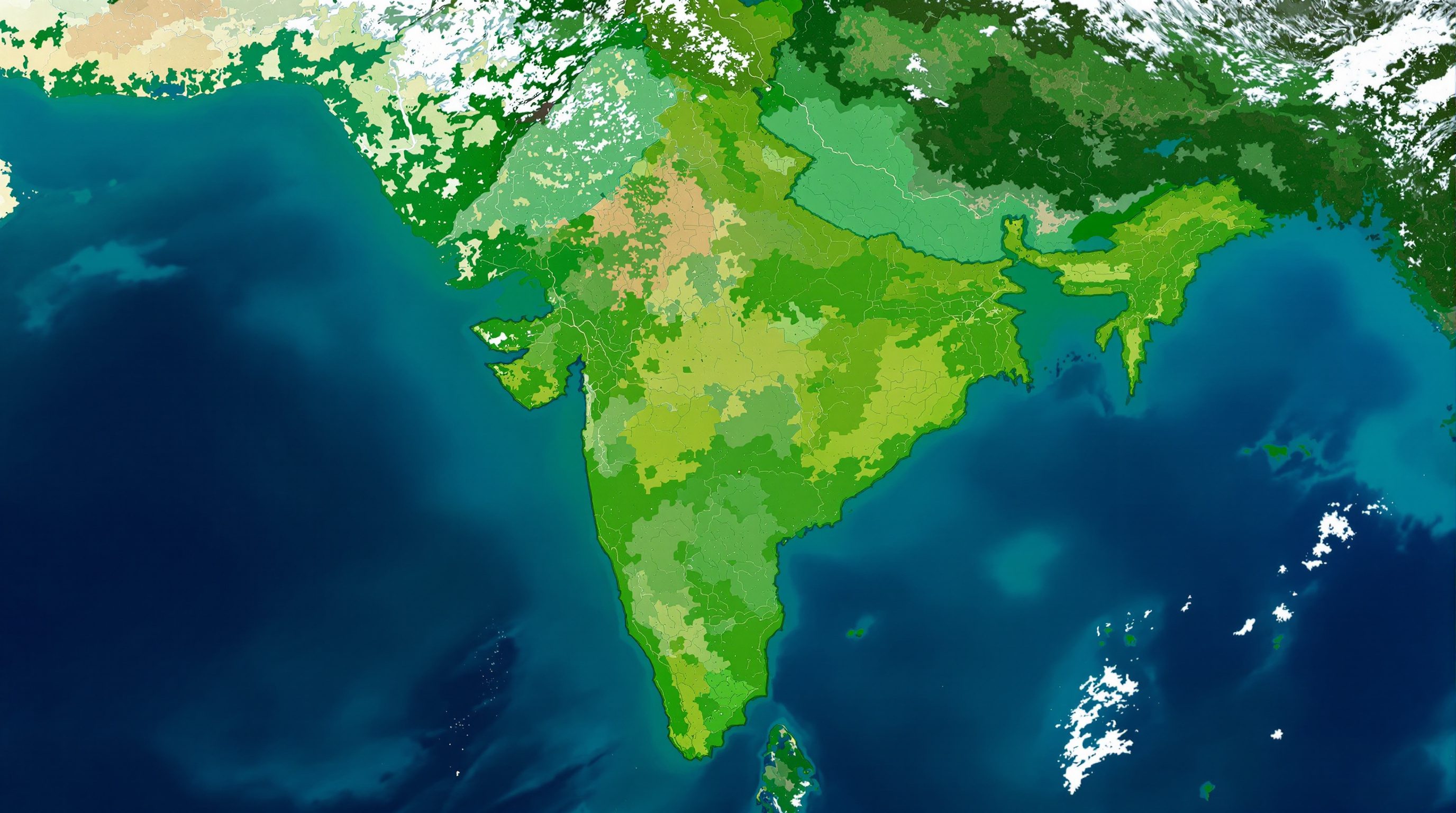
The image looks like a map, but it is not one. It is a grid of millions of pixels, each holding a few brightness numbers - one per spectral band. Your eye can see the parks, but the file does not know where they are; it cannot add up their area or compare this year to last. Classification is the step that turns raw pixels into a map you can count - a layer where every cell carries a label like forest or built-up, ready to be measured, overlaid and argued from.
A crisp coloured map is the most persuasive lie in GIS. The error matrix is the antidote.
From spectral readings to named classes
Every surface reflects sunlight differently across the spectrum. Water swallows most near-infrared light; healthy vegetation reflects a lot of it; concrete and tin roofs are bright almost everywhere. A satellite sensor records these differences as numbers in several bands (wavelength ranges). Two pixels that look the same shade of grey on screen can have quite different band values - and that is what a classifier reads.
Classification is the process of assigning each pixel to a class based on its band values. The output is a new raster where the numbers no longer mean brightness - they mean category: 1 for built-up, 2 for cropland, 3 for forest, and so on. This is what people mean by a Land Use / Land Cover (LULC) map. Strictly, land cover is what is physically there (trees, water, concrete) while land use is what people do with it (a park, a farm, a market); a satellite sees cover directly and infers use, so honest maps say LULC.
The sensor sees cover. Use is a story you add on top - so label it as an inference, not a fact.
Two ways to teach the computer: supervised vs unsupervised
There are two broad routes. In supervised classification, you teach the machine first. You draw small training samples (regions of interest, ROIs) over places you are sure about - this patch is forest, that one is water - and the algorithm learns each class's spectral signature, then labels every other pixel by similarity. A common method is maximum likelihood, which asks 'which class is this pixel most probably in?'
In unsupervised classification, you ask the computer to group pixels into a number of natural clusters by their band values alone (methods like ISODATA or k-means). It hands you, say, 15 spectral clusters with no names; you then inspect them and label each - cluster 4 is water, clusters 7 and 9 are both cropland. Supervised needs field knowledge up front and gives you exactly the classes you want; unsupervised needs no prior labels but leaves the interpretation to the end. Most real projects blend the two.
Choosing classes and imagery that fit the question
Your class list should follow your question, not the other way round. A green-cover study might need only three classes (vegetation, water, everything else); a master-plan base layer needs built-up split from cropland from wasteland. India has a ready reference here: the NRSC national LULC mapping programme classifies the whole country on a standardised, hierarchical scheme - broad Level-I classes such as built-up, agricultural land, forest, wasteland, water bodies and wetlands, each nesting finer sub-classes. Borrowing an agreed scheme means your 'forest' means the same thing as everyone else's.
Resolution decides what you can even attempt. Sentinel-2 (free, 10 m in the key visible and near-infrared bands) resolves individual large plots and neighbourhood green space. Landsat (free, ~30 m) is coarser but reaches back decades - priceless for history. India's own Resourcesat LISS-III (~23.5 m) and AWiFS (~56 m) add regional coverage. A 30 m pixel cannot 'see' a single house or a footpath, so match the sensor to the smallest thing you must map.
The step amateurs skip: accuracy assessment
A classified map always looks convincing - it is crisp and coloured. That is exactly why you must test it. Accuracy assessment compares the map against independent reference points you know the truth for (field visits, high-resolution imagery), and tabulates agreement in an error matrix (also called a confusion matrix). From it you read overall accuracy, plus per-class producer's and user's accuracy, and often the kappa statistic.
The error matrix is honest in a way the map alone is not: it shows which classes get confused (young plantation misread as cropland; bright bare soil misread as built-up) so you can go back, add training samples, and re-run. A LULC map quoted without an accuracy figure is an opinion dressed as a measurement. Report the number, and report how you got it.
'It looks right' is not an accuracy figure. If you cannot state overall accuracy, you have not finished.
NRSC National LULC Mapping
India-wide land-use/land-cover on a standard hierarchical scheme
A ready, agreed class list and reference product for Indian work. nrsc.gov.in
Copernicus Sentinel-2
Free optical imagery, 10 m in key visible/NIR bands
The default free source for fine-grained current LULC; via the Copernicus Data Space Ecosystem.
Resourcesat LISS-III / AWiFS
India's medium-resolution multispectral imagery (~23.5 m / ~56 m)
Regional land/vegetation mapping; free & priced mix via NRSC Bhoonidhi.
ISO 19115
Geographic metadata standard
Record the sensor, date, class scheme and accuracy with the layer, so future users can trust it.
Workshop — classify a slice of your city with Sentinel-2
Produce a small supervised LULC map (built-up, vegetation, water, bare) for a patch of an Indian city, then measure how good it is. Everything here runs on free data.
QGIS (free) + Semi-Automatic Classification Plugin, or ArcGIS Pro + Image Analyst; one free Sentinel-2 scene.
Goal: a 4-class LULC raster + an overall-accuracy figure for a ~5 x 5 km tile
Data: one cloud-free Sentinel-2 scene (free, Copernicus Data Space)
Time: ~90 minutes
- 1Get imagery. Download a recent, cloud-free Sentinel-2 tile for your city from the Copernicus Data Space Ecosystem (free account). In ArcGIS Pro: add the same scene, or pull imagery from a Living Atlas / image service.
- 2Load and composite the bands. In QGIS: install the Semi-Automatic Classification Plugin (SCP), use its band set tool to stack the visible + near-infrared bands. In ArcGIS Pro: use the Image Analyst extension and create a composite/mosaic of the bands.
- 3Draw training samples. In QGIS SCP: create ROIs for each class (several patches per class) and build the spectral signatures. In ArcGIS Pro: open the Training Samples Manager (Classification tools) and digitise samples for the same classes.
- 4Run the classifier. In QGIS SCP: run a maximum likelihood (or minimum-distance) classification to produce the labelled raster. In ArcGIS Pro: run Classify (e.g. Maximum Likelihood or the Support Vector Machine tool) on your training set.
- 5Assess accuracy. Place independent check points (or use a validation ROI set), build the error matrix, and read overall accuracy. In QGIS: SCP's accuracy tool. In ArcGIS Pro: Compute Confusion Matrix. If a class is weak, add samples and repeat step 4.
You’ll walk away with
A four-class LULC raster of your tile, a coloured map, and an honest overall-accuracy percentage - plus the reflex of never publishing a classification without one.
Three altitudes on the same idea
Read the band that fits you — or all three.
Classification gives you a fast, honest read of a site's context fabric. Before a site visit you can quantify how much of the surrounding kilometre is sealed versus green, spot the nearest water body, and see how the neighbourhood has been built out - evidence for a climate-responsive concept. Keep it at the scale it earns: a 10 m map informs siting and massing, never a boundary wall.
LULC is the base layer of statutory planning. Existing-land-use maps for master plans and development plans are, at heart, classifications - and India's AMRUT GIS master-plan and NRSC LULC programmes formalise this. Being able to produce and, crucially, to audit a supplied LULC layer (its classes, date, resolution and accuracy) is core planning literacy: you defend or challenge a land-use figure with the error matrix, not a hunch.
A classified surface turns 'this district feels hard and grey' into a measured share of impervious cover. Combine a built-up/vegetation classification with block boundaries and you can rank streets by greenness, target tree-planting where cover is thinnest, and set a baseline you can re-measure after an intervention.
“The satellite image already is the land-use map - I can just read the areas off it.”
Do it yourself
No software needed - reason about classification for a few minutes.
- 1Name three land classes you would need to answer 'how much of my ward is sealed?' and one pair that a classifier is likely to confuse.
- 2You have only a 30 m Landsat image. List two things in a neighbourhood it cannot reliably map, and why.
- 3Decide: for mapping decade-scale change since 2005, would you choose Sentinel-2 or Landsat, and why?
- 4Sketch a 2x2 error matrix for two classes and mark where the 'misses' (off-diagonal) sit.
- 5Explain in one sentence why 'the map looks correct' is not an accuracy assessment.
The one line to carry out
Peer-reviewed journals & authoritative standards
- 01Lillesand, T., Kiefer, R.W. & Chipman, J. — Remote Sensing and Image Interpretation, 7th ed. — Wiley, 2015.
- 02Jensen, J.R. — Remote Sensing of the Environment: An Earth Resource Perspective, 2nd ed. — Pearson, 2007.
- 03NRSC National Land Use / Land Cover (LULC) Mapping — NRSC / ISRO, ongoing.
- 04National Remote Sensing Centre (NRSC), ISRO — ISRO / Dept. of Space, Govt. of India, ongoing.
- 05Remote Sensing — MDPI, ongoing.
Classification leans on the fact that vegetation behaves unmistakably in the near-infrared - next we turn that single behaviour into a precise number: the vegetation index.
The author
Amogh N P
Architect, interior designer, and creative polymath. Studio Matrx began in his notebooks — his vision of design made honest, useful, and open to everyone. Its Academy is written and taught in his memory, and free, forever.
More about Amogh →