
 Lesson 5.2
Lesson 5.2 · Attractors, Fields & Patterns
Fields & Gradients
Point, line and spin charges merged into a continuous field you can sample anywhere
Stop juggling separate attractors - build one continuous field and sample it anywhere.
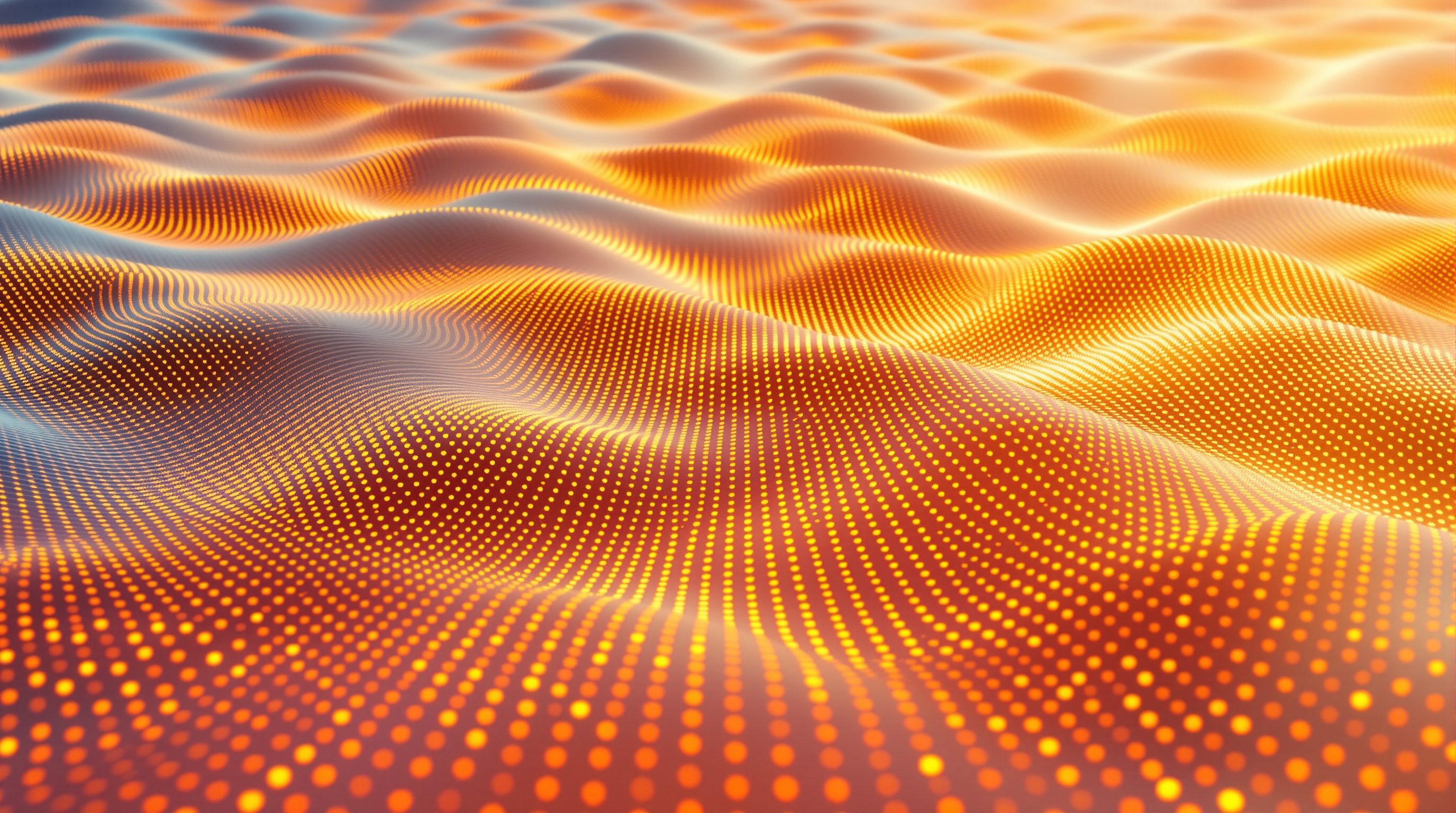
An attractor gives you a single distance. A field gives you a value and a direction at every point in space, summed from as many sources as you like - point charges, line charges, swirling spin forces - all blended into one smooth landscape.
That shift unlocks seamless gradients and true directionality: facades that fade from open to closed with no visible seam, panels that orient themselves to a flow, screens that swirl around a vortex. In this lesson you learn Grasshopper's field family and the two ways to read it - Evaluate Field and field lines.
Charges -> Merge Fields -> Evaluate Field. Length sizes it, direction orients it. Field lines make it visible.
From one attractor to a continuous field
An attractor answers a single question - how far am I from this point? A field answers a richer one - what is the influence here, at any location, from everything at once? Where an attractor gives you one distance per element, a field is a continuous quantity defined everywhere in space: at every point you can ask it for a value or a direction, whether or not any of your geometry sits there.
This is the mental jump of the lesson. Think of a field like temperature in a room or the pull of gravity near several planets: it is smooth, it fills the space, and it is the sum of many sources. Grasshopper has a small but powerful family of field components (the Vector > Field tab) that let you build exactly this - a landscape of force and direction that your geometry can then read.
Fields matter because they compose. Instead of juggling several attractors and manually blending their distances, you drop in several charges, merge them into one field, and sample that single field wherever you like. The blending is handled for you, smoothly, and the result is a continuous gradient rather than a set of separate reactions. It is the difference between three spotlights and one evenly graded wash.
Attractor = one distance. Field = a value/direction defined everywhere, summed from many sources.
The charges: point, line, spin
You build a field from charges, each a source of influence. The Point Charge radiates from a single point; a positive charge pushes outward, a negative one pulls inward, and its strength falls off with distance (you set the charge and the falloff). The Line Charge does the same but radiates from a line segment rather than a point - useful when a whole edge should exert force. The Spin Force is the interesting one: instead of pushing toward or away, it circulates around an axis, creating swirl and vortex patterns that pure attractors cannot.
Each charge on its own is simple; the art is in combining them. That is what Merge Fields does: it takes any number of charges and composes them into one continuous field, adding their influences at every point in space. Two point charges of opposite sign create the classic dipole - flow streaming from one to the other. A ring of charges plus a spin force gives you a weather-system swirl. Because merging is additive and smooth, the seams never show.
Think of the charges as your vocabulary and Merge Fields as the sentence. A designer fluent in fields is really just fluent in what a handful of charge types do and how they add together - the same way an attractor designer is fluent in distance and remap.
Each charge carries a couple of dials worth knowing. The charge value sets how strong the source is and whether it attracts or repels (sign), while the decay or falloff controls how quickly its influence fades with distance - a slow decay reaches far across the surface, a sharp decay stays local. Tuning these per charge is how you balance a composition so no single source dominates, exactly the way you would balance the brightness and throw of several lights in a room.
Point pushes/pulls, Line radiates from an edge, Spin swirls. Merge Fields adds them into one.
Reading the field: Evaluate Field and field lines
A field is invisible until you sample it, and there are two everyday ways to do that. Evaluate Field takes a point (or a whole grid of points) and returns the field's vector there - a direction and a strength. Feed it a grid and you get an arrow at every node, exactly the picture that makes a field legible: arrows pointing along the flow, longer where the field is strong. Those vectors are the useful output - you can use them to move points along the field, orient panels to face the flow, or take just their length as a scalar to drive size or height, folding fields right back into the attractor toolkit from the last lesson.
The second way to see a field is with field lines: streamlines that trace the path a particle would follow if it drifted along the field. Grasshopper's Field Line component starts from seed points and integrates through the field, drawing smooth curves that reveal its structure at a glance - where flow converges, diverges, or spirals. Field lines are both a diagnostic (is my field doing what I think?) and a design output in their own right: those flowing curves can become circulation diagrams, louvre paths, or the ribs of a surface.
Between Evaluate Field (values on a grid) and Field Line (curves through the flow), you have everything needed to turn an abstract field into concrete, buildable geometry.
One habit pays off immediately: sample the field at the same points you will build on. If your panels sit at grid centres, evaluate the field at those centres so each panel gets its own vector - direction and strength aligned exactly to where it lives. Mismatched sampling (evaluating at one set of points, building at another) is the usual cause of a field effect that looks subtly 'off', drifting out of step with the geometry it is supposed to drive.
Gradients and tensor fields across a surface
The reason fields feel so smooth is that they naturally produce gradients - continuous transitions with no visible steps. Sample a merged field across a surface and remap the strengths, and you get a graded quantity - panel depth, colour, aperture - that flows seamlessly from one region to another. This is how you make a facade fade from open to closed, or a screen breathe from dense to sparse, without any abrupt boundary. A gradient is simply a field read as a scalar.
Grasshopper's fields are, more precisely, vector fields - a direction at every point. A related and powerful idea is the tensor field, which carries not just one direction but an orientation with two perpendicular directions at every point (think of the principal stress directions in a shell, or the grain in a piece of wood). Tensor and direction fields are what serious panelization and structural-pattern work rely on: they let a tiling align itself to a meaningful flow across a curved surface rather than being stamped on blindly. You will meet this again with diagrids and gridshells in Module 7.
For now, hold the intuition: a field gives every location both a strength (a gradient you can read as a number) and a direction (a flow you can align to). Most of the expressive power of Module 5 comes from using both at once - strength to size things, direction to orient them.
When to reach for a field - and when not to
Fields are not always the right tool, and part of maturity is knowing when a plain attractor is enough. If you have one focal point and want one property to respond, the Distance-Remap chain from the last lesson is simpler, faster and easier to explain. Reach for fields when you have several sources whose influences should blend smoothly, when you need a genuine direction at every point (to orient panels or draw flow lines), or when you want a continuous gradient across a whole surface rather than a set of independent reactions.
Two honest cautions. First, field components can be heavier to compute than a simple distance measurement - evaluating a dense field on a fine grid takes real time, so sample at the resolution you actually need. Second, a field is still a visual construct: it looks physical, but a Grasshopper Spin Force is not wind and a Point Charge is not the sun. If you need true airflow or structural stress you go to a simulation or an analysis engine (Kangaroo, Karamba, Ladybug), and you use the field for the design language, not the physics.
With that boundary clear, fields become one of the most elegant tools you have: a way to make an entire surface respond, smoothly and directionally, to a composition of sources you can arrange like lights in a room.
Point Charge
Field source radiating from a point, strength falling off with distance
Positive pushes out, negative pulls in. The basic building block of a field.
Spin Force
Field source that circulates around an axis
Creates swirl and vortex patterns no distance-based attractor can produce.
Merge Fields
Component that composes several charges into one continuous field
Adds influences smoothly at every point - your separate sources become a single field.
Evaluate Field
Component returning the field vector at a given point or grid
How you sample a field: direction and strength you can use to move, orient or size geometry.
Field Line
Component tracing streamlines through a field from seed points
Makes the invisible flow visible; also a design output (paths, ribs, circulation).
Workshop - a dipole facade gradient
You will build a small field from two opposite charges and a spin force, sample it across a wall, and use it to drive both panel size and panel rotation - the canonical field exercise.
Rhino + Grasshopper. Components: Point Charge, Spin Force, Merge Fields, Evaluate Field, Field Line, Vector Length, Remap Numbers, Orient/Rotate.
Goal: a continuous field driving size (strength) and orientation (direction) across a wall
Inputs: a rectangular surface, two Rhino points, one axis for spin
Time: ~40 minutes
- 1Place two Point Charges at your two points - one positive, one negative - to form a dipole. Add a Spin Force on a vertical axis between them for a little swirl.
- 2Wire all three into Merge Fields to compose one continuous field. Panel the output to confirm it is a single field object.
- 3Divide your wall surface into a grid of points and feed them into Evaluate Field. You now get one vector per grid point - direction and strength.
- 4Use the vector length (Vector Length), remapped, to drive the radius or size of a panel at each point; use the vector direction to Rotate or Orient the panel so it faces the flow.
- 5Add a Field Line component seeded along one edge to draw streamlines through the field, and lay them over the facade as a diagnostic - do the panels align with the flow you see?
You’ll walk away with
A live definition plus two images: the facade coloured/sized by field strength, and the same facade with field lines overlaid showing the flow. A sentence on where you placed the charges and what architectural idea they represent.
Three altitudes on the same idea
Read the band that fits you — or all three.
Fields let you compose influence the way you compose a plan. Place charges at the entrances, the cores, the worst solar corners, add a spin force for movement, merge them, and read one continuous gradient across the whole envelope. You get a facade that transitions smoothly and directionally instead of reacting in separate patches - and a single, editable diagram behind it that you can defend.
A gradient is the most sophisticated thing a repeating element can do. A field lets a ceiling, screen or floor pattern flow from dense to open across a room with no hard line, and its direction can align slats or tiles to the way people move through the space. It reads as considered and calm - the opposite of a stamped, uniform grid - and still cuts cleanly on a machine.
Fields are where you show you have moved past copied attractor definitions. Anyone can drop a point and remap distance; building a merged field, sampling it with Evaluate Field, and drawing field lines demonstrates real command of vectors and data. Show one field driving both size (its strength) and orientation (its direction) - that pairing tells a reviewer you understand what a vector field actually is.
“A Grasshopper field is a physics simulation - it models real forces like wind or magnetism.”
Do it yourself
Think about direction, not just distance.
- 1In one sentence, how does a field differ from a single attractor?
- 2Name the three charge types and say what each one does to the flow.
- 3What does Evaluate Field return at a point, and what are the two things you can do with it?
- 4What are field lines, and give one use for them beyond diagnostics.
- 5When is a plain attractor the better choice than a full field?
The one line to carry out
Peer-reviewed journals & authoritative standards
- 01Mode Lab - The Grasshopper Primer (Third Edition) — grasshopperprimer.com, 2020.
- 02Rutten, D. - The Guide to Grasshopper (community) — grasshopper3d.com, 2026.
- 03Pottmann, Asperl, Hofer, Kilian - Architectural Geometry — Bentley Institute Press, 2007.
- 04Grasshopper Docs - component reference — grasshopperdocs.com, 2026.
Fields give us smooth, continuous variation. Next we turn to the other great source of parametric richness - _discrete_ structure: the grids, Voronoi cells, triangulations and hex tilings that divide a surface into panels you can then vary with exactly the attractors and fields you have just learned.
The author
Amogh N P
Architect, interior designer, and creative polymath. Studio Matrx began in his notebooks — his vision of design made honest, useful, and open to everyone. Its Academy is written and taught in his memory, and free, forever.
More about Amogh →